Erasing Integrated Learning : A Simple yet Effective Approach for Weakly Supervised Object Localization
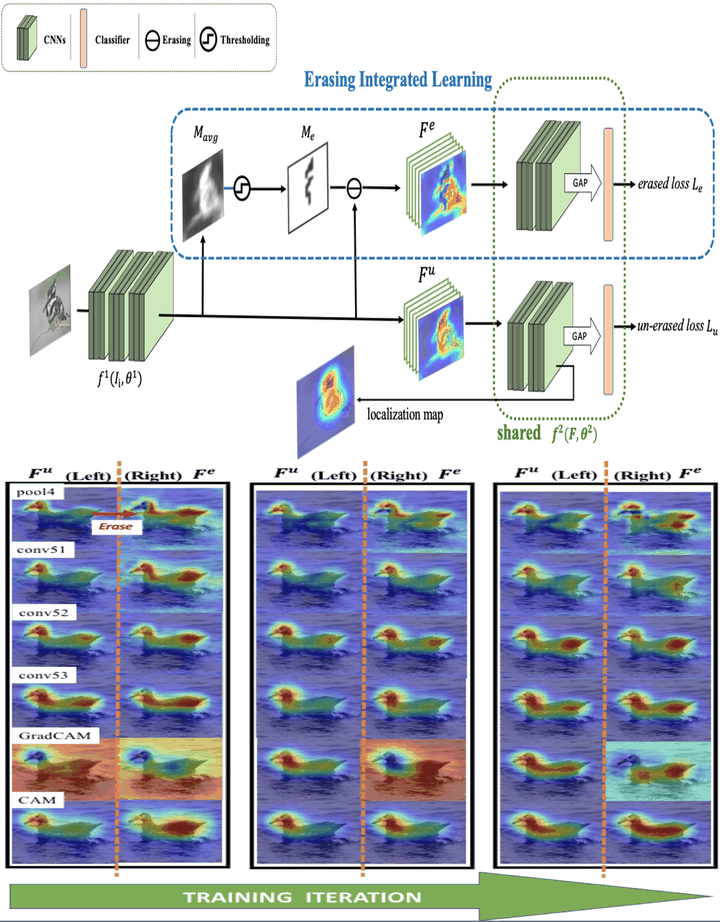
 When EIL is inserted at a feature map, an average map $M_{avg}$ is first produced by channel-wise average pooling. With thresholding $M_{avg}$ to obtain an erasing mask $M_{e}$, the erased feature map $F^{e}$ by $M_{e}$ and the unerased $F^{u}$ are fed into the network again under a shared dual-branch treatment.
Formally, we denote the training image set as $I=\{\{I_i,y_i\}\}^N_{i=1}$, where $y_i=\{1,2,...,C\}$ is the label of the image $I_i$, $C$ is total classes of images and $N$ is the amount of images. Let $\theta$, lowercase $f$, and uppercase $F$ denote network parameters, functions, and feature maps, respectively.
The network $f^1(I,\theta^1)$ before EIL is applied can produce the original unerased feature map, which is denoted as $F^{u}\leftarrow f^1(I_i,\theta^1)$ and $F^{u}\in\mathcal{R} ^ {K \times H \times W}$, where $K$ stands for the number of channels, $W$ and $H$ for the width and height, respectively. We make use of $F^{u}$ as self-attention to generate the erasing mask. Specifically, we compress $F^{u}$ into an average map $M_{avg}\in\mathcal{R} ^ {1 \times H \times W}$ through channel-wise average pooling. Then we apply a hard threshold $\gamma$ on $M_{avg}$ to produce the erasing mask $M_e\in\mathcal{R} ^ {1 \times H \times W}$, in which the spatial locations of those pixels having intensity greater than $\gamma$ are set to zero. We perform the erasing operation by doing spatial-wise multiplication between unerased feature map $F^{u}$ and mask $M_{e}$, to produce the erased feature map $F^{e}\in\mathcal{R} ^ {K \times H \times W}$.
Afterwards, both the unerased feature map $F^{u}$ and the erased counterpart $F^{e}$ are fed into the latter part of the network $f^2(F,\theta^2)$ together. As these two data streams are processed by the same function $f^2$ and parameters $\theta^2$, such structure can be regarded as a dual-branch network of shared weights. More specifically, $f^2(F,\theta^2)$ produces class activation maps (CAM) \cite{zhou2016learning}, applies global average pooling \cite{lin2013network} on CAM and utilizes a fully connected layer followed by softmax operation to get the prediction score $p$ for each branch, with $p^{u}$ and $p^{e}$ for the erased and the unerased, respectively. In the end, the classification losses from the two branches will be added up to calculate the total loss $\mathcal{L}$. Note that we also introduce a loss weighting hyperparameter $\sigma$ to control the relative importance between the unerased loss $\mathcal{L}^{u}$ and the erased loss $\mathcal{L}^{e}$.
\begin{algorithm}
    \SetAlgoLined
    \KwInput{Input image $I=\{\{I_i,y_i\}\}^N_{i=1}$ from $C$ classes, erasing threshold $\gamma$, weighting hyperparameter $\sigma$}
    \While {training is not convergent}{
    Calculate the feature map $F^{u}\leftarrow f^1(I_i,\theta^1)$ \;
    Calculate the average map $M_{avg}=\frac{\sum^K_{i=1}F^{u}_i}{K}$\;
    Calculate the erasing mask $M_{e_{i,j}}=\begin{cases}
                                    0, &\quad if\ M_{avg_{i,j}}\ge \gamma\\
                                    1, &\quad else\\
                                \end{cases}$\;
    Get the erased feature map $F^{e}=F^{u}\otimes M_{e}$ \;
    Calculate prediction of $F^{e}$: $p^{e}\leftarrow f^2(F^{e},\theta_2)$ \;
    Calculate prediction of $F^{u}$: $p^{u}\leftarrow f^2(F^{u},\theta_2)$ \;
    Obtain erased loss: $\mathcal{L}_{e}=-\frac{1}{C}\sum_c y_{i,c} log(p^{e}_c)$ \;
    Obtain unerased loss:$\mathcal{L}_{u}=-\frac{1}{C}\sum_c y_{i,c} log(p^{u}_c)$\;
    Calculate the total loss: $\mathcal{L}=\mathcal{L}_{u}+\sigma \mathcal{L}_{e}$ \;
    Back-propagate and update parameters $\theta^1$, $\theta^2$ \;
    }
     \caption{Training algorithm for EIL}
     \label{al:1}
\end{algorithm}